
Camera Tuning Guide#
To create visually good images from the raw data provided by the camera sensor, a lot of image processing takes place. This is usually done inside an ISP (Image Signal Processor). To be able to do the necessary processing, the corresponding algorithms need to be parameterized according to the hardware in use (typically sensor, light and lens). Calculating these parameters is a process called tuning. The tuning process results in a tuning file which is then used by libcamera to provide calibrated parameters to the algorithms at runtime.
The processing blocks of an ISP vary from vendor to vendor and can be arbitrarily complex. Nevertheless a diagram of common blocks frequently found in an ISP design is shown below:
+--------+
|  Light |
+--------+
    |
    v
+--------+     +-----+    +-----+    +-----+    +-----+    +-------+
| Sensor |  -> | BLC | -> | AWB | -> | LSC | -> | CCM | -> | Gamma |
+--------+     +-----+    +-----+    +-----+    +-----+    +-------+
Light The light used to illuminate the scene has a crucial influence on the resulting image. The human eye and brain are specialized in automatically adapting to different lights. In a camera, this has to be done by an algorithm. Light is a complex topic and to correctly describe light sources you need to graph the spectrum of the light. To simplify things, lights are categorized according to their color temperature (K). This is important to keep in mind as it means that calibrations may differ between light sources even though they have the same nominal color temperature.
For best results the tuning images need to be taken for a complete range of light sources.
Sensor The sensor captures incoming light and converts the measured analogue signal to a digital representation in the form of raw images. The light is commonly separated into red, green and blue channels by a color filter array. As these filters are not perfect, postprocessing needs to be done to recreate the correct colors.
BLC Black level correction. Even in perfect darkness a sensor produces pixel values above zero. This is due to two system artifacts that impact the measured light levels on the sensor. Firstly, a deliberate and artificially added pedestal value is added to get an evenly distributed noise level around zero to avoid negative values and clipping the data.
Secondly, underlying electrical noise can be caused by various external factors. These include thermal noise as well as electrical interference.
To get good images with true blacks, this ‘black level’ needs to be subtracted. Where the black level is known for a sensor, it is hardcoded in libcamera and needs no further calibration. If needed, that value can be manually overwritten in the tuning configuration process.
AWB Auto white balance. For a proper image displaying true colors, the color channels may need to be adjusted to attain the correct white balance. This makes monochrome objects in the scene appear monochrome in the output image (white is white and gray is gray). In the libipa implementation of libcamera, this is managed by a grey world model, so no tuning is necessary for this step.
LSC Lens shading correction. The lens in use has a big influence on the resulting image. The typical effects on the image are lens-shading (also called vignette). Due to the physical properties of lenses, the transmission of light through the lens will decrease around its circumference. To make things even more complicated, the magnitude of this effect can vary depending on the light’s color or wavelength. Because of this LSC needs to be tuned for multiple light sources, as well as each color channel individually.
CCM Color correction matrix. After the previous processing stages, we find that although the grays are preserved, the colors are still not correct. This is mostly due to the color temperature of the light source, and imperfections in the color filter array within the sensor. To correct for this a ‘color correction matrix’ is calculated. This 3x3 matrix, is used to optimize the captured colours by minimizing the perceived color error. To do this, images of a chart of known and precisely measured colors are captured, usually using a macbeth chart. The matrix itself is calculated using linear optimization to map each measured colour of the chart to its known value. The colour error is measured in deltaE.
Gamma Gamma correction. Today’s displays usually apply a gamma of 2.2 to the image they show. For images to be perceived correctly by the human eye, they need to be encoded with the corresponding inverse gamma. See also <https://en.wikipedia.org/wiki/Gamma_correction>. This block doesn’t need to be tuned, but is crucial to consider when displaying images correctly.
Materials needed for the tuning process#
Precisely calibrated optical equipment is very expensive and out of the scope of this document. However, it is still possible to get reasonably good calibration results at little cost. The most important devices needed are:
A light box with the ability to produce defined light of different color temperatures. Typical temperatures used for calibration are 2400K (incandescent), 2700K (fluorescent), 5000K (daylight fluorescent), 6500K (daylight). As a first test, keylights for webcam streaming can be used. These are available with support for color temperatures ranging from 2500K to 9000K and can be combined with a simple white or grey card box. It is important that the box is of neutral grey color, so that it doesn’t influence the measurements. For better results professional light boxes are needed.
A ColorChecker chart. These are sold from calibrite. It makes sense to get the original one, as there is no other easy way to recreate this with similar quality.
A integration sphere. This is used to create completely homogenious light for the lens shading calibration. We had good results with the use of a large light panel with sufficient diffusion to get an even distribution of light (the above mentioned keylight).
An environment without external light sources. Ideally calibration is done without any external lights in a fully dark room. A black curtain is one solution, working by night is the cheap alternative.
Overview of the process#
In libcamera, the tuning process consists of the following steps:
Capture images for each tuning step at multiple color temperatures
Configure the tuning process
Run the tuning script to create a tuning file
Taking raw images with defined exposure/gain#
For all the tuning files you need to capture a raw image with a defined exposure time and gain. It is crucial that no pixels are completely saturated on any channel. At the same time the images should not be too dark. Once you have an image you think is ok to use, you can check if the image is too dark by doing a dry run through the tuning tool to make sure it accepts your image. If it doesn’t, you’ll need to adjust the exposure time and gain.
Make sure you adjust BOTH the exposure time and the analogue gain to achieve this. Different constant exposure files will be needed for each calibration image. You can check if any pixels are over exposed using a histogram analyser in tools such as camshark, or viewing the output .dng files in RAW viewers such as Rawtherapee or Darktable. If there are any peaks near the far right of the graph, the image is overexposed (see below).
The most saturated pixels in the image should be within the white square on the Macbeth color chart. You’ll need to be careful that your light source itself is not in the image causing parts of the image to be over saturated.
Strive for an exposure time such that the brightest pixel is roughly 90%
saturated. Finding the correct exposure time is currently a manual process, so
it is recommended to use a live preview from the camera to adjust the exposure
accordingly. This can be found in tools such as Camshark, or by examining the
captured images in tools such as Rawtherapee or Darktable. After finding the
correct exposure time, the easiest way to capture a raw image is with the
cam application that gets installed with libcamera.
Create a constant-exposure-<temperature>.yaml file with the following content:
frames:
  - 0:
      AeEnable: false
      AnalogueGain: 1.0
      ExposureTime: 1000
(N.B. Please make sure to change the exposure time and the analogue gain to the correct value for each color temperature to ensure the image is adequately exposed)
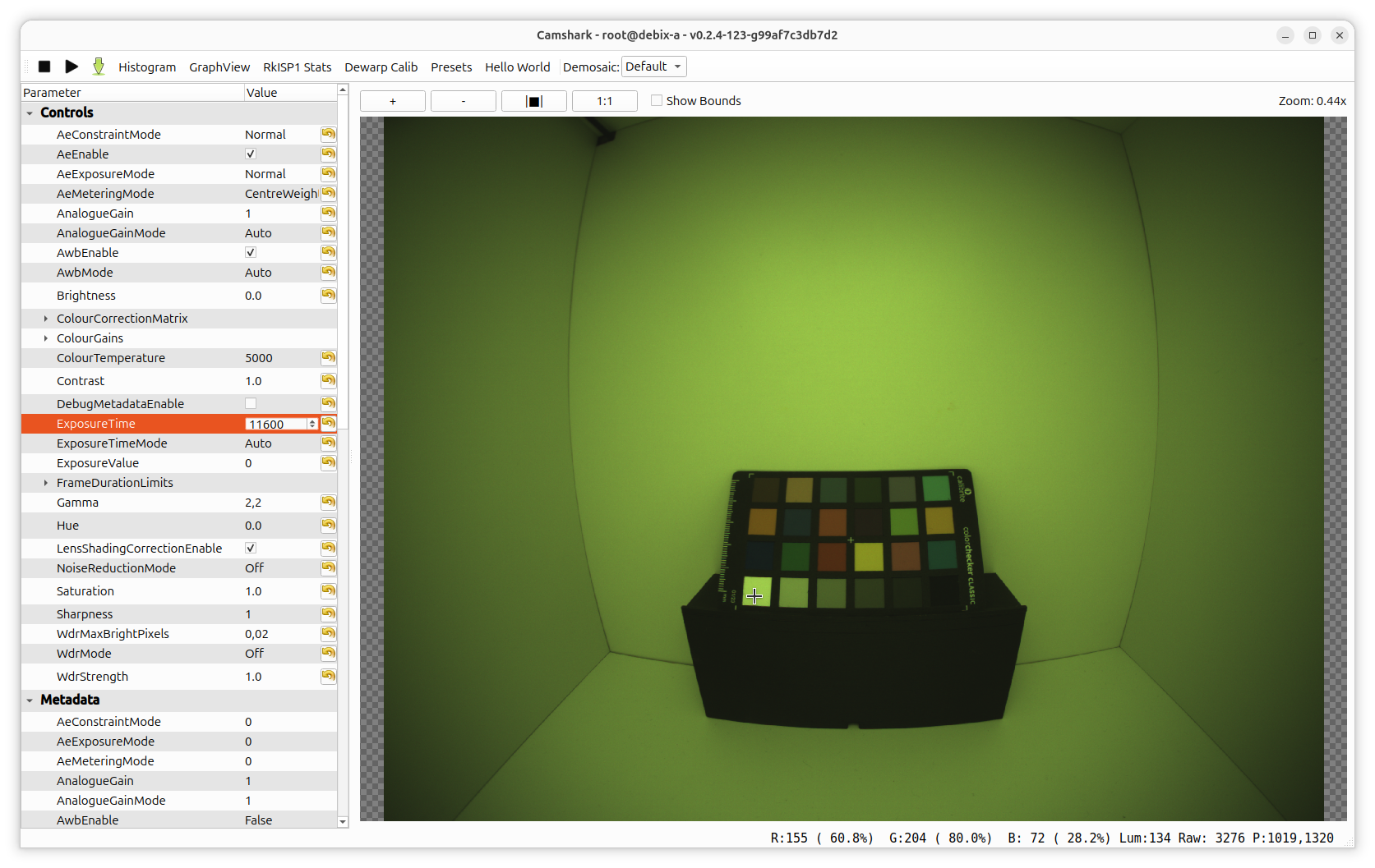
A well exposed image. No pixels are over-exposed on any channel.#
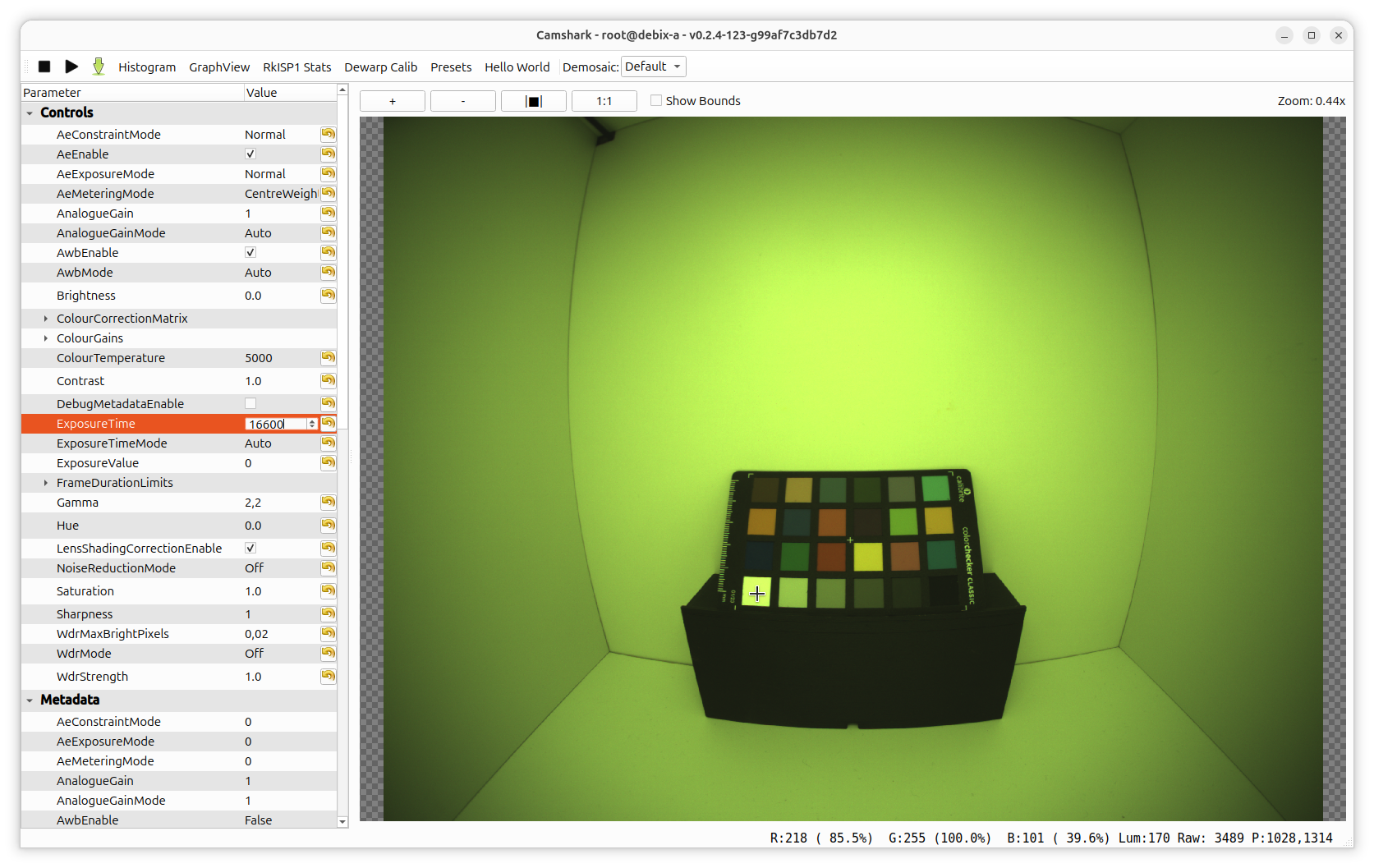
An over-exposed image. The white square on the Macbeth color chart is over-exposed.#
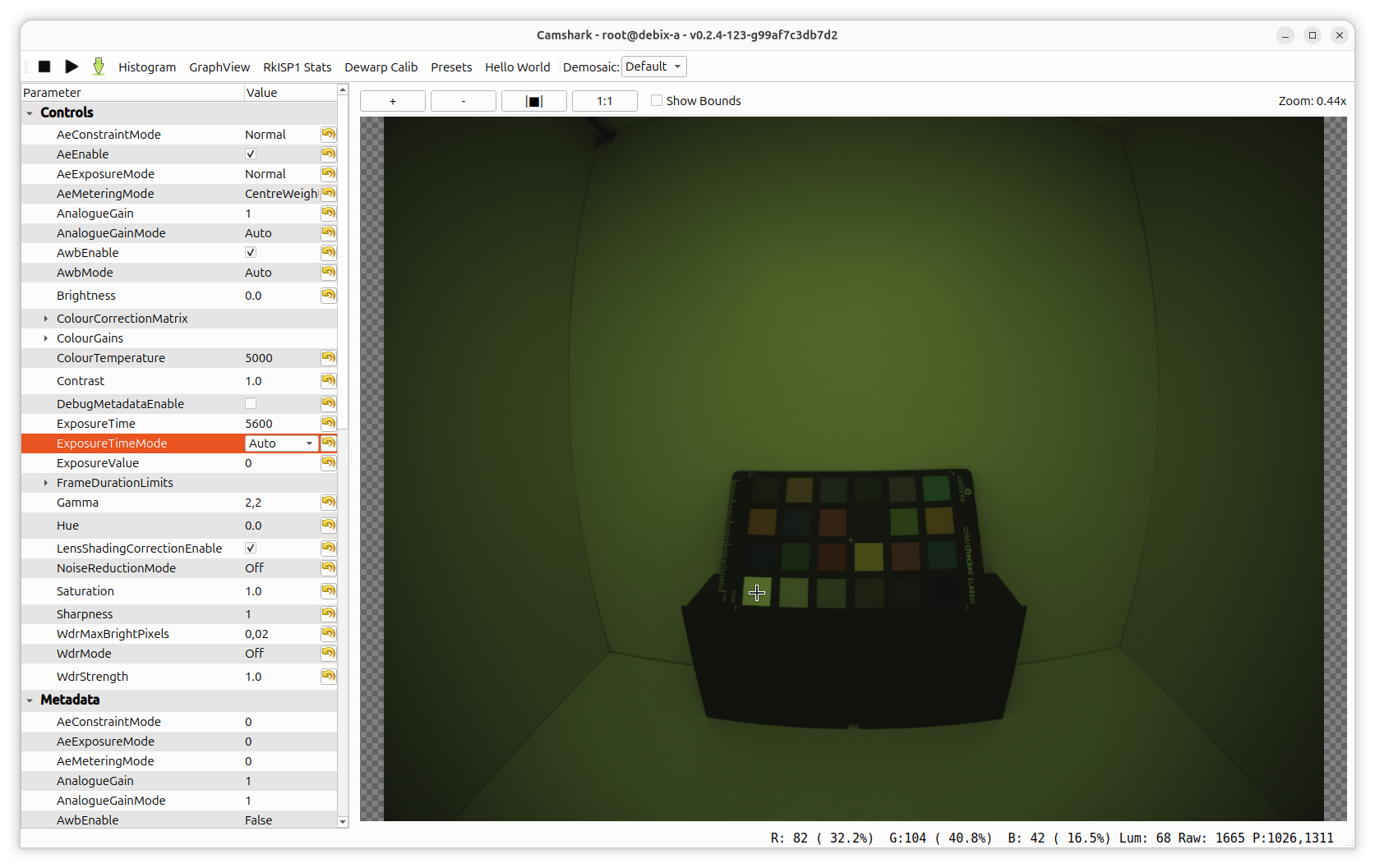
An under-exposed image.#
Ideally, the AnalogueGain should be set to 1.0 and only the ExposureTime should be adjusted. It is also important that the AnalogueGain is not set to any value less than 1.0.
- Next, capture one or more images using the following command:
cam -c 1 --script constant-exposure-<temperature>.yaml -C -s role=raw --file=image_#.dng
Note
Typically the brightness changes for different color temperatures. So this has to be readjusted for every color temperature.
Capture images for lens shading correction#
To be able to correct lens shading artifacts, images of a homogeneously lit neutral gray background are needed. Ideally an integration sphere is used for that task.
If an integration sphere is not available, images of a flat panel light can be used. If there are multiple images for the same color temperature, the tuning scripts will average the tuning results which can further improve the tuning quality.
Note
Currently lsc is ignored in the ccm calculation. This can lead to slight color deviations and will be improved in the future.
Images shall be taken for multiple color temperatures and named
alsc_<temperature>k_#.dng. # can be any number, if multiple images are
taken for the same color temperature.
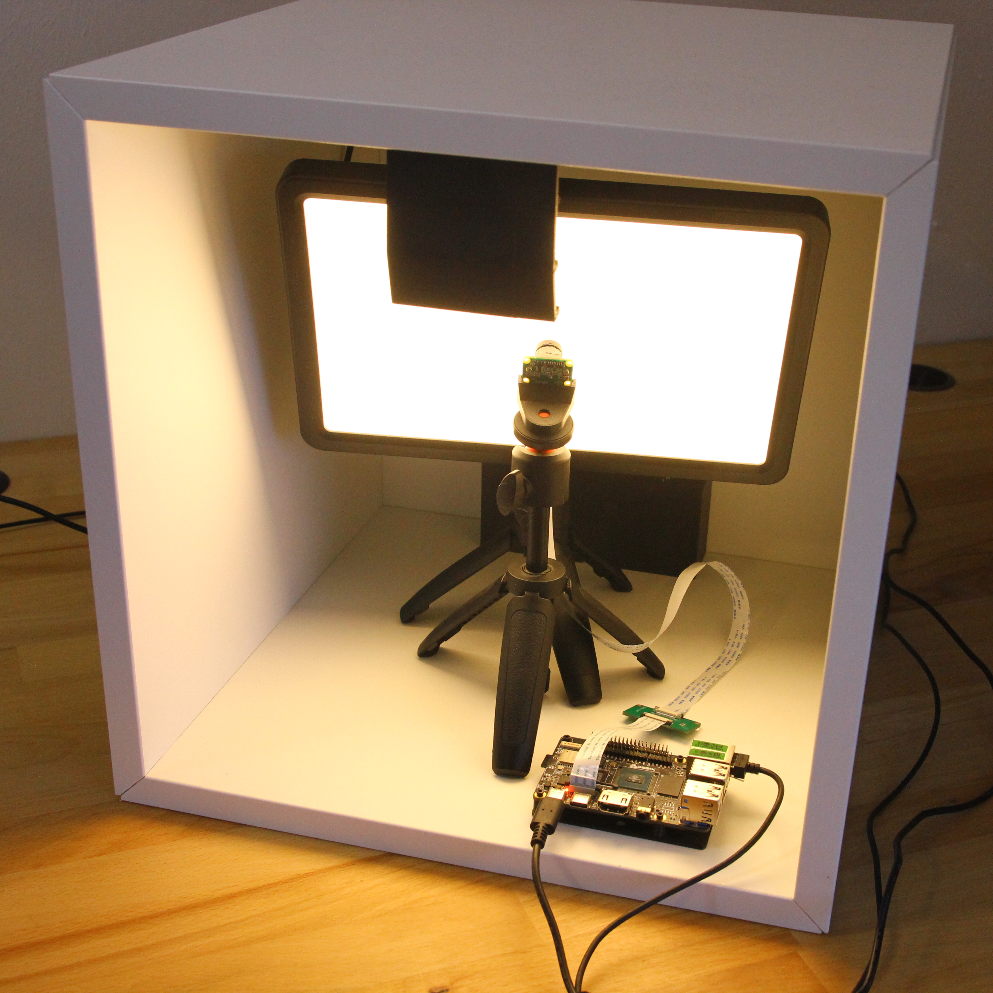
Sample setup using a flat panel light. In this specific setup, the camera has to be moved close to the light due to the wide angle lens. This has the downside that the angle to the light might get way too steep.#
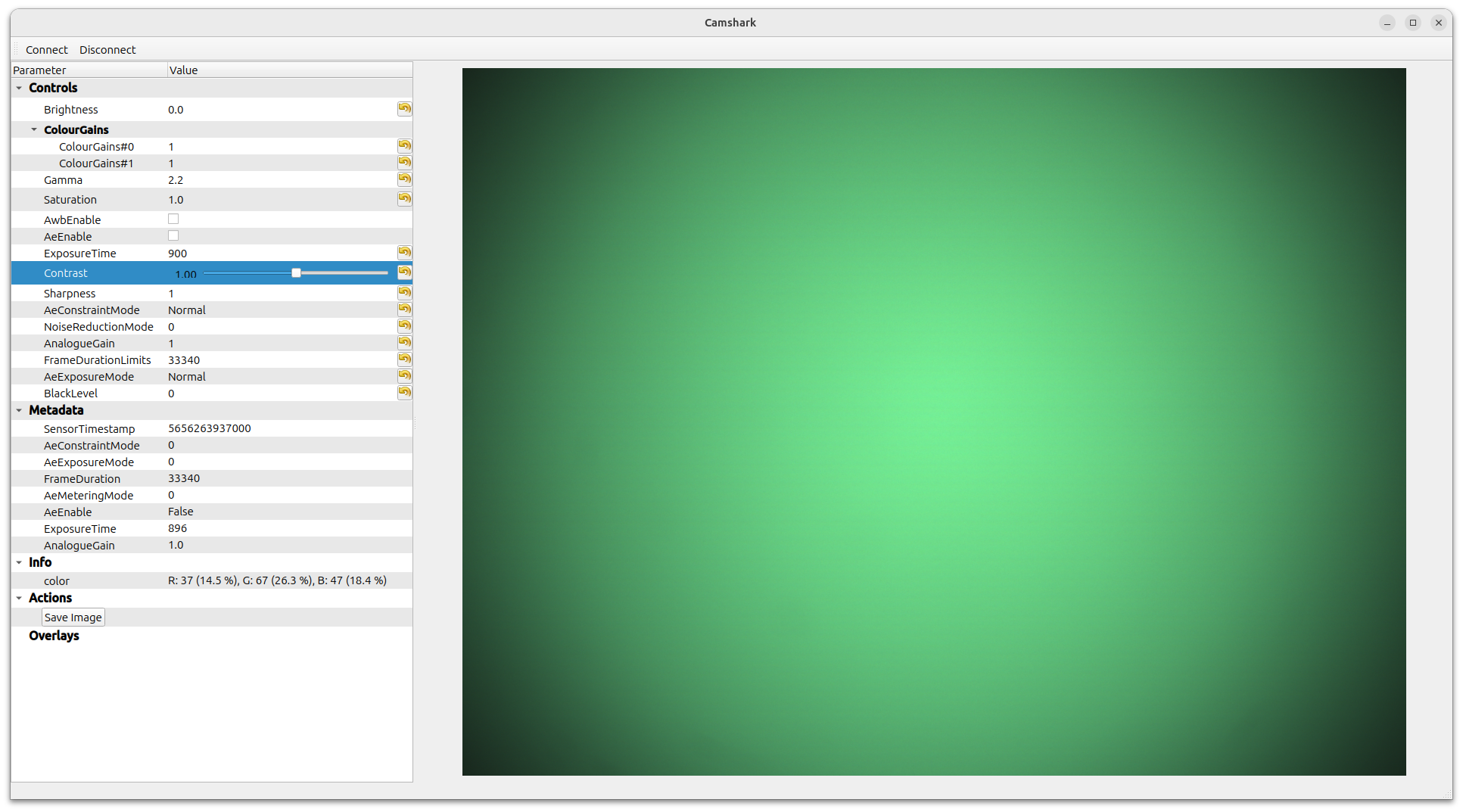
A calibration image for lens shading correction.#
Ensure the sensor is fully lit. Especially with wide angle lenses it may be difficult to get the full field of view lit homogeneously.
Ensure that the brightest area of the image does not contain any pixels that reach more than 95% on any of the colors (can be checked with camshark).
- Take a raw dng image for multiple color temperatures:
cam -c 1 --script constant-exposure-<temperature>.yaml -C -s role=raw --file=alsc_3200k_#.dng
Capture images for color calibration#
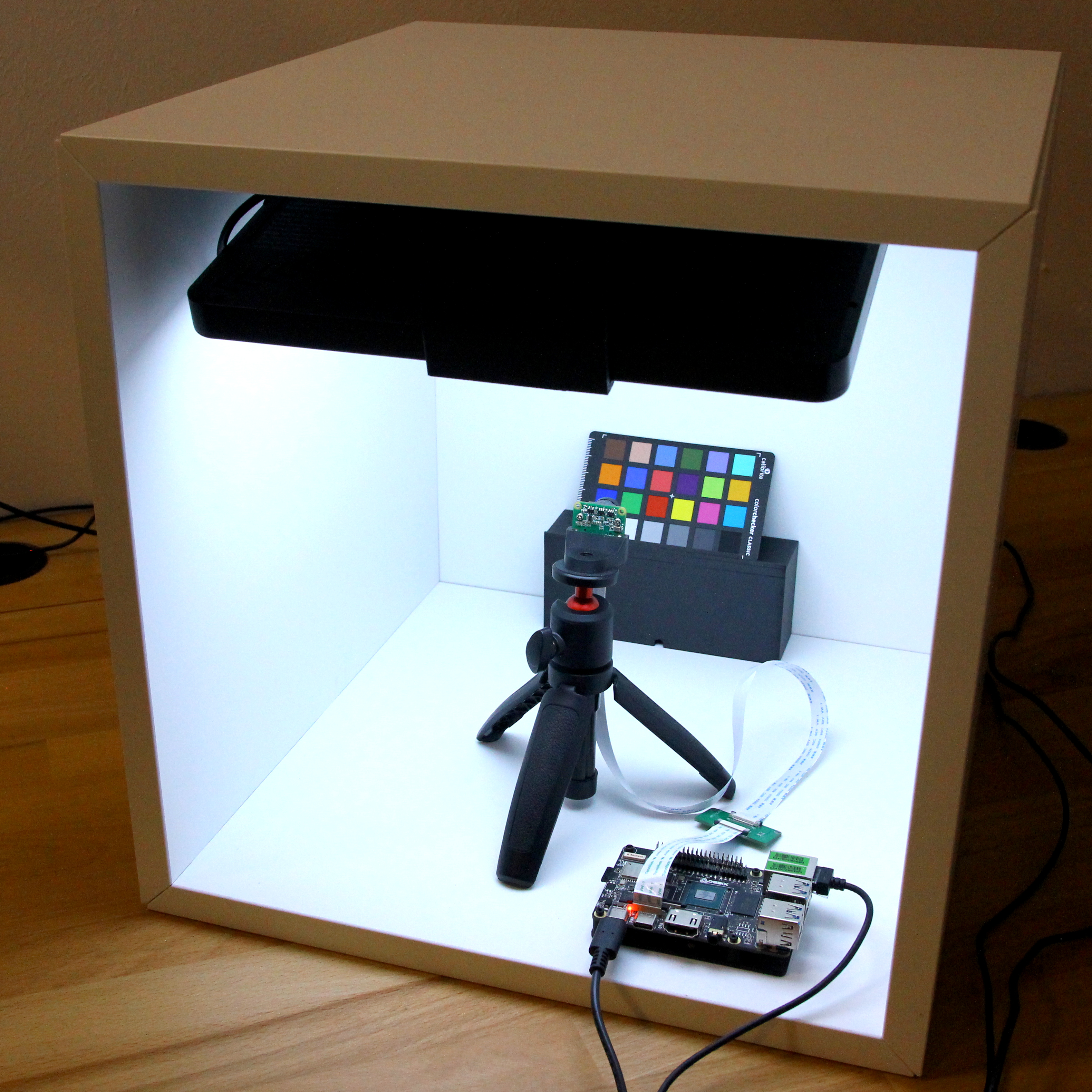
To do the color calibration, raw images of the ColorChecker chart need to be
taken for a range of different light sources. These need to be named
<sensor_name>_<lux-level>l_<temperature>k_0.dng.
- For best results the following hints should be taken into account:
Ensure that the 18% gray patch (third from the right in bottom line) is roughly at 18% saturation for all channels (a mean of 16-20% should be fine). This can be achieved either by changing the exposure time or the intensity of the light source.
Ensure the color checker is homogeneously lit (ideally from 45 degree above)
No stray light from other sources is present
The color checker is not too small and not too big (so that neither lens shading artifacts nor lens distortions are effecting the color chart)
The best way currently to find this information is to use Camshark. There, you can use the Viewfinder mode to see the saturation levels of each of the R, G, and B channels. You can also see the mean saturation level of the 18% gray patch by hovering the mouse cursor over it.
If no lux meter is at hand to precisely measure the lux level, a lux meter app on a mobile phone can provide a sufficient estimation.
Run the tuning scripts#
After taking the calibration images, you should have a directory with all the tuning files. It should look something like this:
../tuning-data/
├── alsc_2500k_0.dng
├── alsc_2500k_1.dng
├── alsc_2500k_2.dng
├── alsc_6500k_0.dng
├── imx335_1000l_2500k_0.dng
├── imx335_1200l_4000k_0.dng
├── imx335_1600l_6000k_0.dng
The tuning scripts are part of the libcamera source tree. After cloning the libcamera sources the necessary steps to create a tuning file are:
- ::
# Install system prerequisites sudo apt install python3-pip libexiv2-dev libboost-python-dev
# Install the necessary python packages cd libcamera python -m venv venv source ./venv/bin/activate pip install -r utils/tuning/requirements.txt
# Create a default config cp utils/tuning/config-example.yaml config.yaml
# Run the tuning script utils/tuning/rkisp1.py -c config.yaml -i ../tuning-data/ -o tuning-file.yaml
After the tuning script has run, the tuning file can be tested with any
libcamera based application like qcam. To quickly switch to a specific tuning
file, the environment variable LIBCAMERA_<pipeline>_TUNING_FILE is helpful.
E.g.:
LIBCAMERA_RKISP1_TUNING_FILE=/path/to/tuning-file.yaml qcam -c1
Sample images#
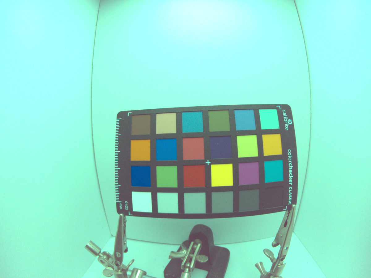
Image without black level correction (and completely invalid color estimation).#
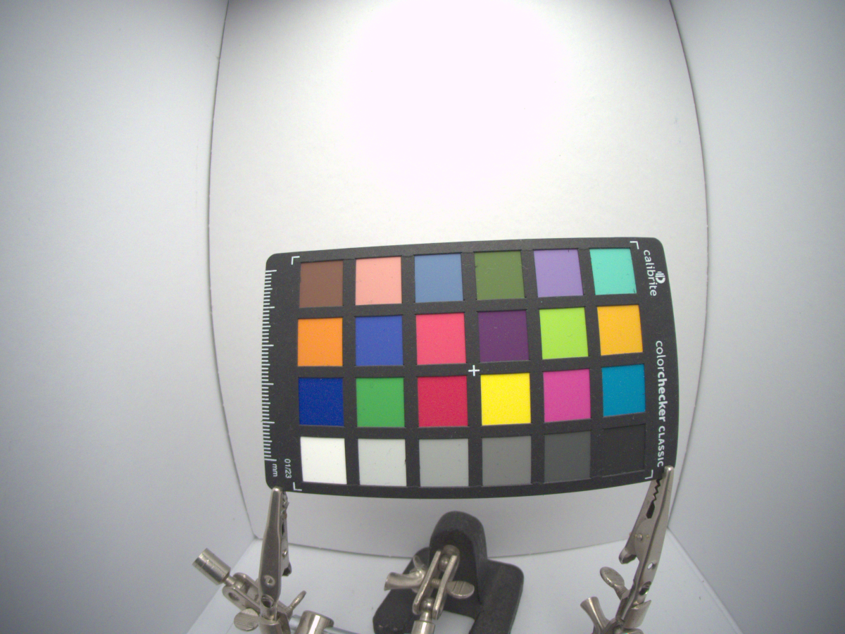
Image without lens shading correction @ 3000k. The vignetting artifacts can be clearly seen#
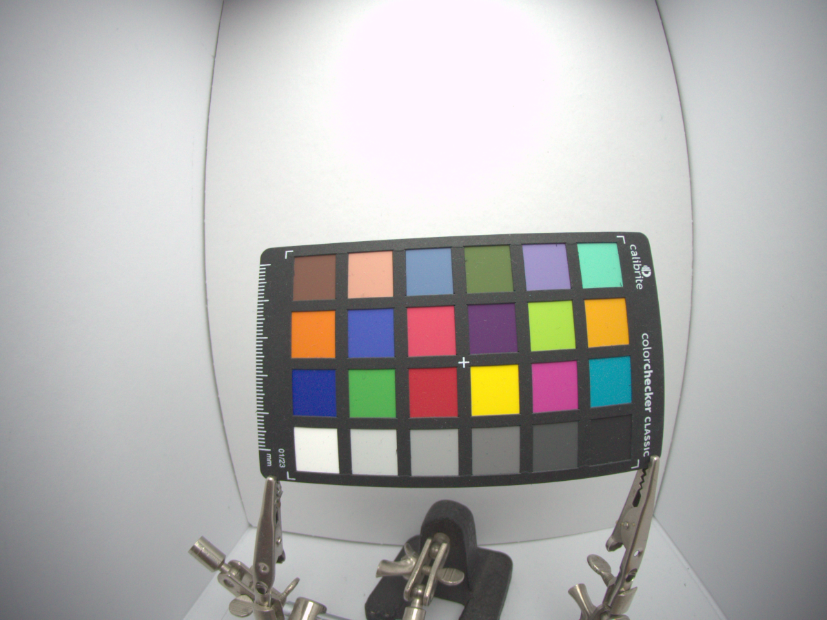
Image without lens shading correction @ 6000k. The vignetting artifacts can be clearly seen#
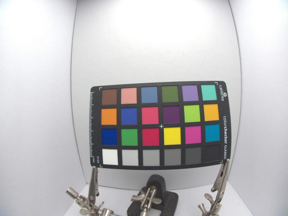
Fully tuned image @ 3000k#
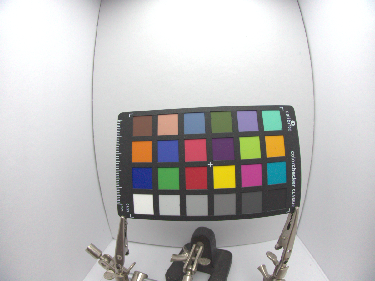
Fully tuned image @ 6000k#